GPU programming with Triton, part 1

Most of us start using GPUs through a framework. We move a model to the device, training runs faster, and for a long time that is all we need to know. The difficulty begins when something is slower than it should be and we have no way to reason about why, because the GPU has been a black box the whole time.

This series is our attempt to open that box. In this series, we will learn how a GPU executes code, write kernels for it in Triton, and measure everything we write. Triton is a domain-specific language (DSL) for GPU kernels that is embedded in Python, and it comes with both a compiler and a runtime. We will learn more about what that means towards the end of this part. We chose Triton because it lets us write fast GPU kernels without requiring us to start with NVIDIA CUDA® C++. However, writing efficient GPU kernels starts with understanding the fundamentals: how GPUs execute work, organize threads, and move data through memory.

This first part therefore focuses primarily on GPU fundamentals, building the foundation we need before we start writing kernels in Triton. We will start with a single line of PyTorch code, creating a simple tensor on the GPU and adding it to another, and ask what the GPU actually executes when that line runs.

From there we step into CUDA C++, where every detail of GPU programming is explicit: how threads are organized, how work is distributed, and how data moves between the CPU, the GPU, and the levels of memory in between. Seeing those mechanics directly is the best way to appreciate what Triton takes care of for us. We finish by writing the same kernel in Triton and comparing the two side by side.

One line of PyTorch

Let’s start with a simple PyTorch example and follow what happens when it reaches the GPU:

import torch
 
a = torch.randn(1_000_000, device="cuda")
b = torch.randn(1_000_000, device="cuda")
c = (a + b).relu()

‍The first two lines create tensors containing one million random numbers each and place them in GPU memory. The third line looks simple: add the two tensors, then apply a ReLU.

From Python’s point of view, this is a single expression. But what does the GPU actually execute?

It executes two separate programs, called kernels.

A kernel is a GPU function, one that the GPU typically executes across different elements in parallel. The CPU asks the GPU to run a kernel, and that request is called a kernel launch. Here, the word kernel has nothing to do with an operating-system kernel or the small matrix used in a convolution; in GPU programming it simply means a function the GPU executes.

When PyTorch evaluates a + b, it launches one kernel that reads a and b, adds their elements, and writes the result. It then evaluates .relu() by launching a second kernel, which reads that intermediate result, replaces negative values with zero, and writes the final output.

So, one line of PyTorch becomes two GPU kernel launches.

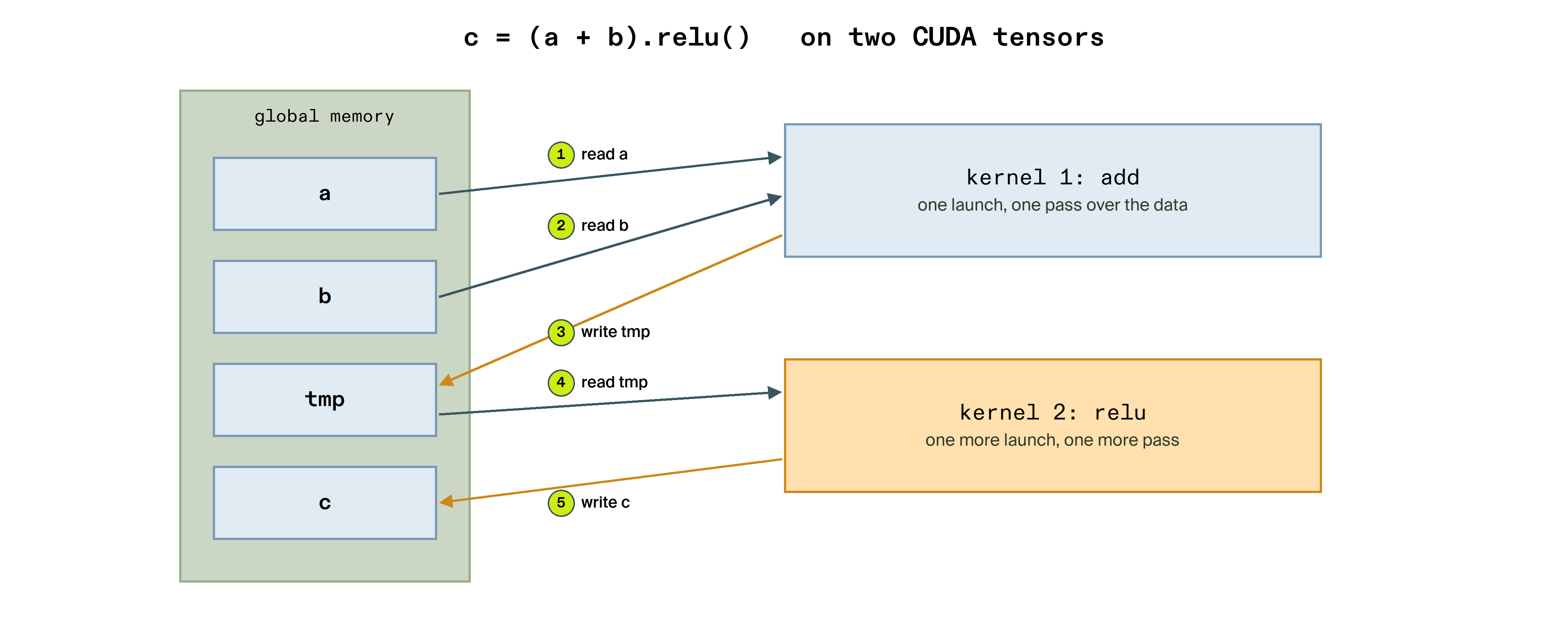
The first kernel reads a and b, adds them, and writes the result back to GPU memory as an intermediate tensor, tmp. The second kernel then reads tmp, applies ReLU, and writes the final result to c.

If we count those memory operations, we get five array-sized trips through global memory:

1. Read a
2. Read b
3. Write tmp
4. Read tmp
5. Write c

The actual computation, however, only needs the values from a and b to produce c. If the addition and ReLU could happen together, we would need only three array-sized memory operations: read a, read b, and write c. The extra write and read of tmp happen because the addition and ReLU are executed as separate kernels.

Why does PyTorch do this? In its default eager mode, PyTorch executes each operation as Python reaches it. When it launches the addition, PyTorch does not look ahead and optimize it together with the ReLU that follows. It executes the addition as its own operation and writes the result to GPU memory. When Python reaches .relu(), PyTorch launches another kernel, which reads that intermediate result and produces the final output.

Later, we will see what happens when these two operations are brought together into a single kernel, eliminating the intermediate write and read through global memory.

Counting the kernels

We can see this directly using PyTorch's profiler, which records the GPU kernels executed by our code:

import torch
from torch.profiler import ProfilerActivity, profile

def add_relu(a, b):
    return (a + b).relu()

a = torch.randn(1_000_000, device="cuda")
b = torch.randn(1_000_000, device="cuda")

# Warm up once so one-time initialization stays out of the trace.
add_relu(a, b)
torch.cuda.synchronize()

with profile(activities=[ProfilerActivity.CPU, ProfilerActivity.CUDA]) as prof:
    add_relu(a, b)
    torch.cuda.synchronize()  # wait for the GPU before ending the trace

print(prof.key_averages().table(sort_by="cuda_time_total", row_limit=12))

Before we see what this prints, let’s first understand the code above. The first call to add_relu() and the torch.cuda.synchronize() immediately after it are simply a warm-up, so we can ignore them for now. They make sure one-time initialization work is completed before we start profiling.

Inside the profiler, we call torch.cuda.synchronize() again. GPU operations are asynchronous, meaning the CPU continues on to its next statement while work is still running on the GPU, so without this call the profiling region could end before the kernels we want to observe have completed. The call blocks the CPU until every queued GPU operation has finished. We will explore asynchronous execution in more detail once we write a kernel of our own.

Here is the table this printed on our NVIDIA L40S GPU on Crusoe (the GPU we are using for the purpose of this series), with the CPU timing columns omitted for space:‍‍

Name                                                      Self CUDA   # of Calls
--------------------------------------------------------  ----------  ----------
aten::add                                                  3.680us            1
void at::native::vectorized_elementwise_kernel<4, at...    3.680us            1
aten::relu                                                 0.000us            1
aten::clamp_min                                            2.976us            1
void at::native::vectorized_elementwise_kernel<4, at...    2.976us            1
cudaLaunchKernel                                           0.000us            2
cudaDeviceSynchronize                                      0.000us            2
--------------------------------------------------------  ----------  ----------
Self CUDA time total: 6.656us

At first glance, the profiler output can look a bit busy because it mixes high-level PyTorch operations with the actual GPU kernels they trigger. To break it down:

• PyTorch operations: Rows like aten::add, aten::relu, and aten::clamp_min are framework-level calls.
• Hardware kernels: The two rows starting with vectorized_elementwise_kernel are the actual routines executed on the GPU.

The first GPU kernel handles the addition in 3.680 us. For ReLU, PyTorch routes through clamp_min under the hood, running a second kernel that takes 2.976 us. You might notice that aten::relu logs 0.000 us of self-time; the profiler assigns GPU time to the innermost leaf operation (clamp_min) that actually fires the kernel, rather than parent wrappers like aten::relu.

There is an even simpler way to confirm the count. The cudaLaunchKernel row shows 2 calls, meaning PyTorch asked CUDA to launch exactly two kernels. That matches what we saw in the diagram: one kernel for the addition and another for ReLU.

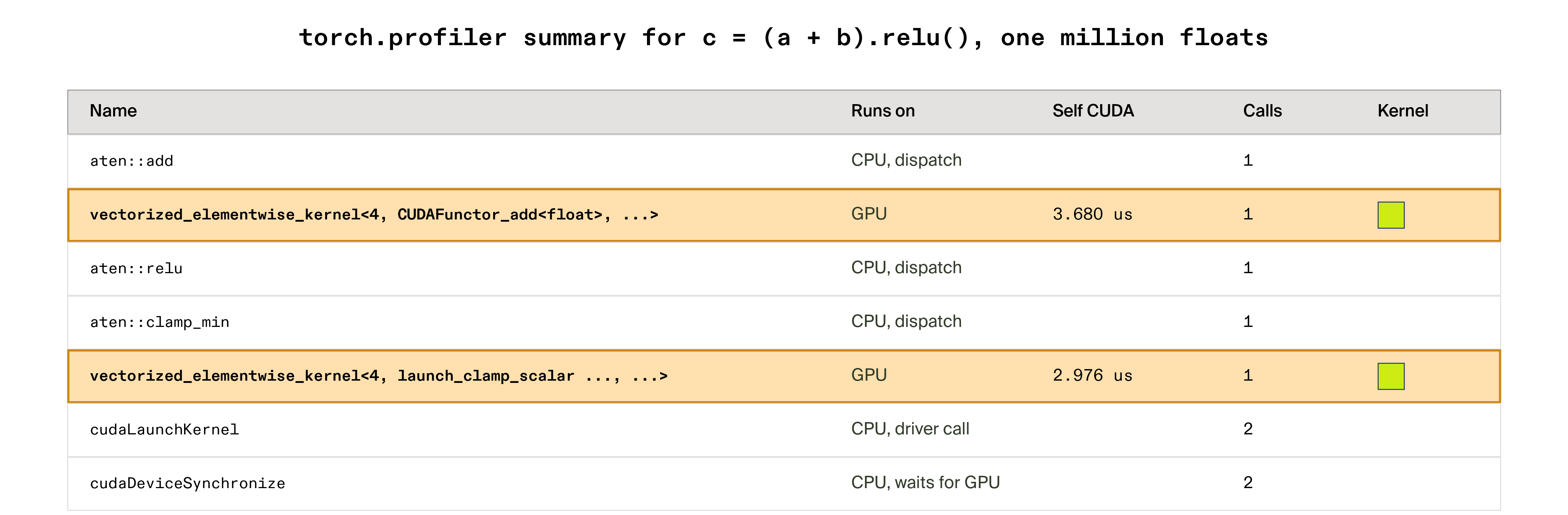
The exact kernel names are not important, and they can change between PyTorch versions. The important takeaway is: our single Python expression resulted in two GPU kernel launches.

Now that we can see what PyTorch is asking the GPU to execute, the next step is to understand how the GPU actually executes that work. For that, we need to look at how a GPU is built.

Why a GPU is built the way it is

Suppose we want to double every element of an array of one thousand numbers. The elements are independent: e.g., doubling the 5th element in the array needs nothing from the 4th element. So instead of one processor visiting the elements in turn, we can give each element to its own worker and finish in a single step. This is data parallelism: one operation carried out simultaneously on many independent data elements. When the pieces need no coordination at all, the work is often called embarrassingly parallel. Elementwise operations such as addition and ReLU have exactly this shape, and when heavier workloads like matrix multiplication, convolution, and attention are broken down into thousands of smaller parallel computations, they follow this exact same paradigm, which is why deep learning maps so well onto a GPU. GPUs are well suited for such parallel processing, where the same operation needs to take place on a different set of data.

But not everything does. Summing an array to a single value forces partial results to be combined, which introduces dependencies between workers. Operations like this are called reductions, they need a different strategy, and we will see them later in the series.

That design goal shows up in the GPU hardware. A CPU is built for low latency on a small number of instruction streams. It has a few large cores, sophisticated control logic, big caches, branch prediction and out-of-order execution all aimed at making one thread run fast. A GPU is built for throughput, completing a large amount of work per unit time, and spends its silicon on thousands of simple arithmetic units running in parallel instead.

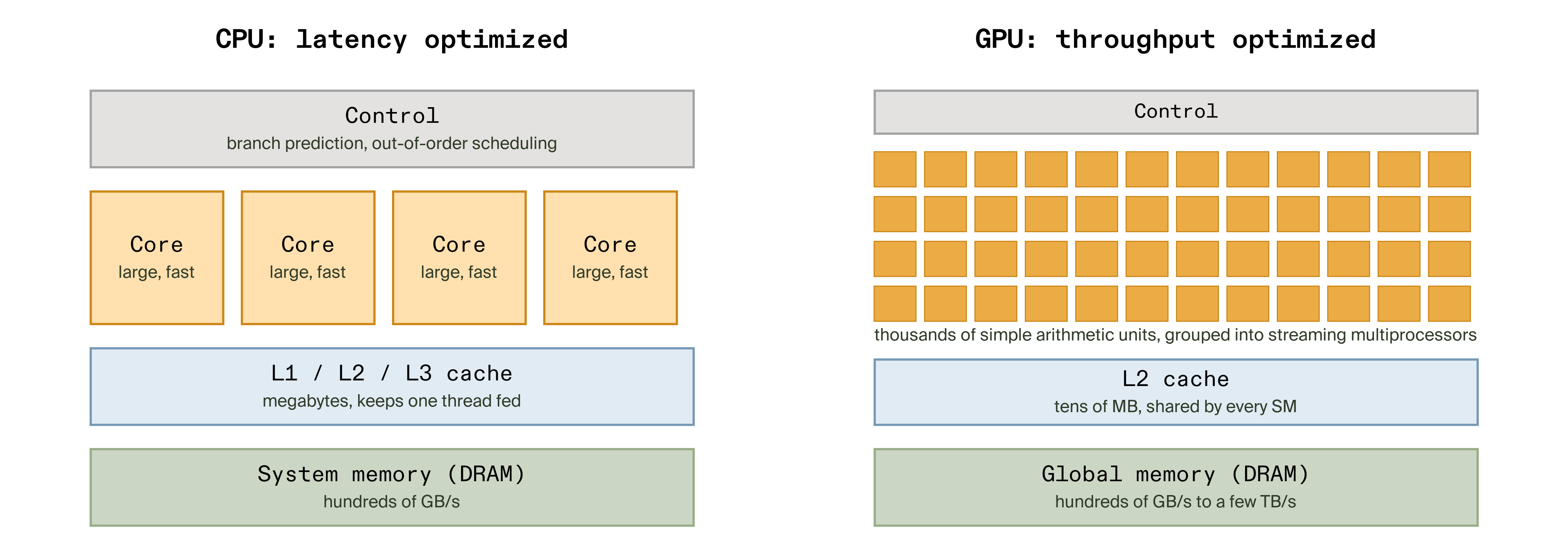
We now have an intuition for why a GPU is designed around massive parallelism. The next question is how we give it work to do, and to answer that let’s write our first GPU kernel.

A first CUDA program

CUDA is NVIDIA's platform for programming its GPUs. It extends C++ with a few keywords and a special function-call syntax, and it comes with a compiler, nvcc, that produces a program containing both CPU code and GPU code. In CUDA's vocabulary, the CPU is the host and the GPU is the device, and we will use those two words from here on.

The worker we have been describing has a proper name in CUDA: a thread. A thread runs the kernel's instructions on its own piece of the data. Here is a small kernel that shows threads in action. It computes nothing; each thread simply announces itself with a print statement:

#include <cstdio>

__global__ void hello_kernel() {
    // threadIdx.x is this thread's position inside its block, 0 to 7 here.
    printf("hello from thread %d\n", threadIdx.x);
}

int main() {
    hello_kernel<<<1, 8>>>();   // one block of eight threads
    cudaDeviceSynchronize();    // wait for the GPU before main() returns
    return 0;
}

If you know C++, two parts of this program probably look unusual: __global__ and the <<<...>>> syntax. They are CUDA extensions to C++, understood by NVIDIA's nvcc compiler. __global__ tells the compiler that a function is a GPU kernel, while <<<...>>> tells the CUDA runtime how that kernel should be launched on the GPU. Neither is part of standard C++ syntax.

1. __global__ marks a GPU kernel: The keyword __global__ marks hello_kernel as a kernel, meaning the host launches it and the device executes it. A CUDA kernel does not return a value directly to the host. Kernels that produce results typically write them to memory, where the host or another kernel can access them later.
2. <<<1, 8>>> launches the kernel: The launch syntax <<<1, 8>>> is how the host asks the GPU to run the kernel. The two numbers specify how many groups of threads to create and how many threads each group should contain. CUDA calls a group of threads a block, so here we are launching one block containing eight threads.
   There is no loop in the kernel, yet its body runs once for each of the eight threads. Instead of writing a loop that processes eight items one after another, we launch eight threads and let the GPU execute them in parallel. We will have much more to say about blocks once we need more than one of them; for now, a single block is enough.‍
3. threadIdx.x identifies a thread within the block: The built-in variable threadIdx.x tells each thread its position inside the block, from 0 to 7 here. Every thread runs the same kernel code, but threadIdx.x has a different value for each one. That index is often part of how a thread determines which piece of data it should work on.

We compile the program with nvcc and run the result like any other executable:

nvcc -O2 -arch=native -o 01_hello_kernel 01_hello_kernel.cu
./01_hello_kernel

‍On our machine, this produced:

hello from thread 0
hello from thread 1
hello from thread 2
hello from thread 3
hello from thread 4
hello from thread 5
hello from thread 6
hello from thread 7

‍The lines happened to appear in order on our machine, but CUDA does not guarantee that ordering. Threads execute concurrently, and a correct GPU program should never depend on the order in which individual threads happen to run or produce output.

We launched eight threads here, but the GPU does not treat them as eight completely independent pieces of work. To understand what happens next, we need to introduce one of the most important concepts in GPU execution: the warp.

How the hardware runs threads

We have been describing threads as if each one were an independent worker. The hardware is a little more structured than that. On NVIDIA GPUs, threads are organized into warps of 32. The 32 threads of a warp execute each instruction together, and each thread applies that instruction to its own data. NVIDIA calls this execution model SIMT (Single Instruction Multiple Threads).

Our block contains only eight threads, so it still occupies one warp. Of the warp's 32 lanes, only eight are active for our block and the remaining 24 are inactive. This is our first hint that the number of threads we choose for a block can affect how efficiently the hardware is used. When a block contains more than 32 threads, its threads are divided into multiple warps; a block of 256 threads, for example, is eight warps, and those warps are then scheduled for execution by the GPU.

The part of the GPU that schedules and executes warps is called an SM (Streaming Multiprocessor). A GPU contains many SMs, and the exact number depends on the GPU. The NVIDIA L40S GPU we are using has 142 SMs.

For comparison, the NVIDIA A100 Tensor Core GPU has 108 SMs, while the NVIDIA H100 Tensor Core GPU has 132 SMs in the SXM version and 114 SMs in the PCIe version. Each SM contains execution units along with the storage its threads need: registers, a small on-chip memory, and caches. We will look at each of these when we reach the memory hierarchy; for now it is enough to know that an SM is where warps run.

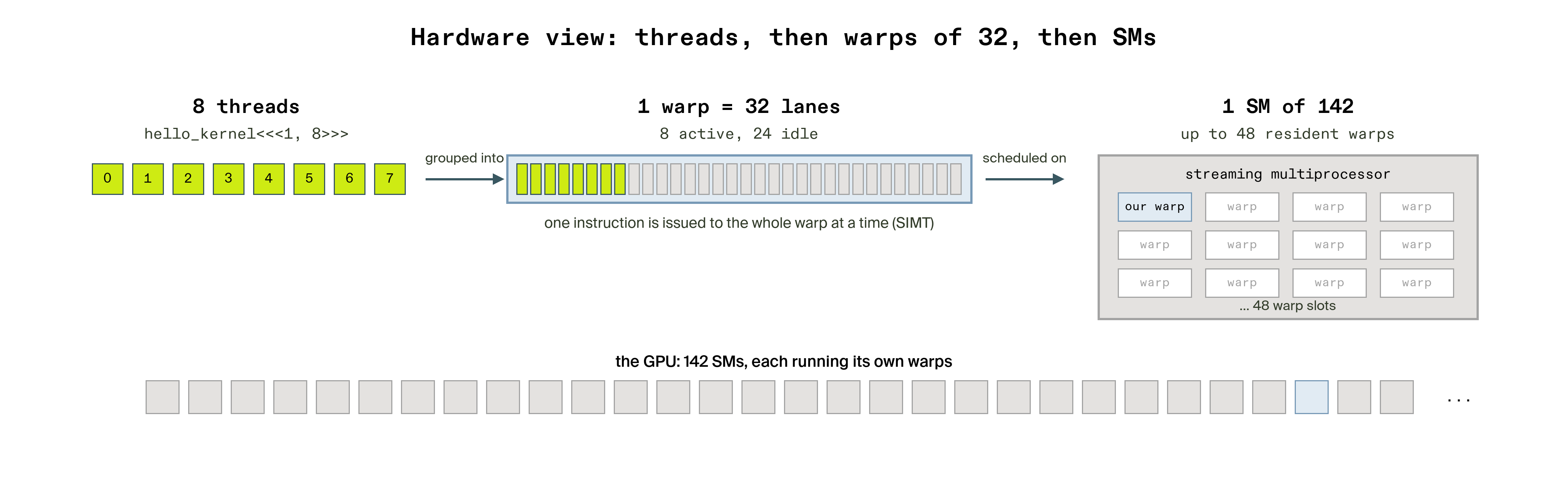
Because NVIDIA GPUs use warps of 32 threads, CUDA block sizes are commonly chosen as multiples of 32. We will see why choices such as 128, 256, or 512 threads per block appear so often as we write larger kernels.

Squaring an array: two memories

A kernel that only prints is not much use. To do real work, a kernel has to read inputs and write outputs, and that brings us to the most important structural fact about a GPU program: the host and the device have separate memories. The CPU uses the system's main memory, while the GPU has its own global memory. Neither processor can read the other's memory directly, so data has to be copied across the PCIe bus in both directions.

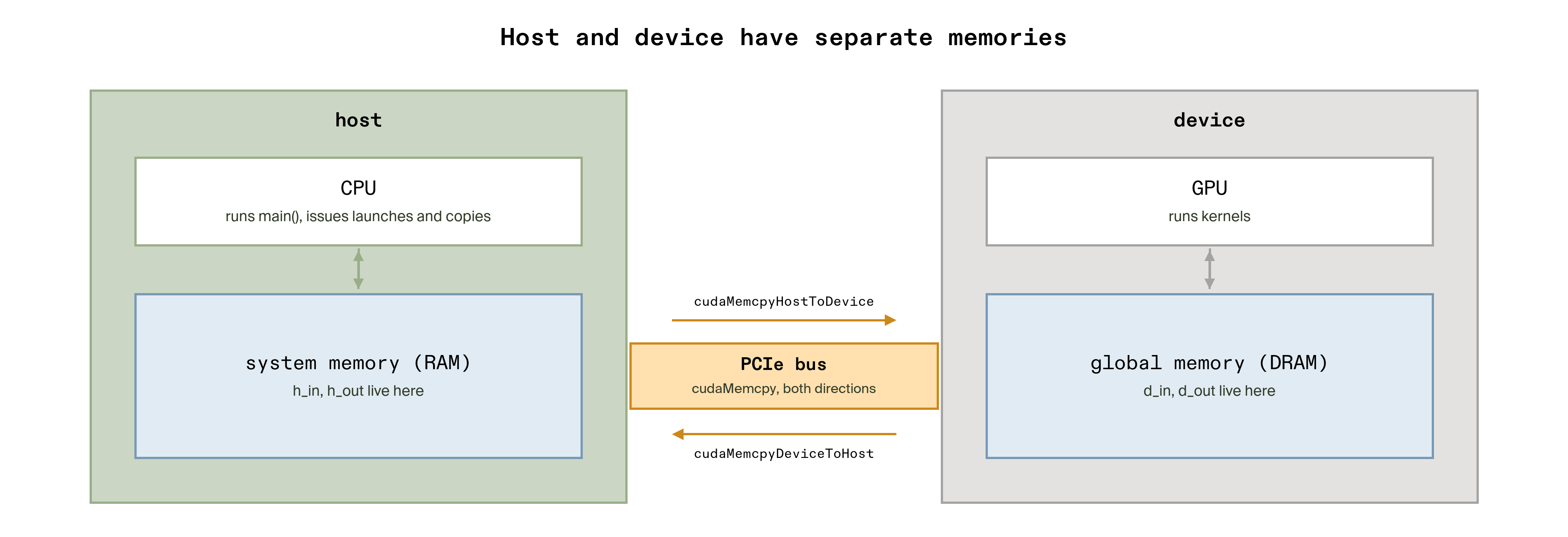
For our first example, we will use the basic explicit-memory workflow:

1. Allocate memory on the device
2. Copy the input from host to device
3. Launch the kernel
4. Copy the result from device back to host
5. Free the device memory

Here is that workflow in a program that squares eight numbers, using one thread per number:

#include <cstdio>

__global__ void square_kernel(const float* in, float* out, int n) {
    int i = threadIdx.x;      // one block: thread index = element index
    if (i < n) {              // never touch memory past the array's end
        out[i] = in[i] * in[i];
    }
}

int main() {
    const int n = 8;
    const size_t bytes = n * sizeof(float);
    float h_in[n], h_out[n];                            // host arrays
    for (int i = 0; i < n; ++i) h_in[i] = (float)(i + 1);

    float *d_in = nullptr, *d_out = nullptr;            // device pointers
    cudaMalloc(&d_in, bytes);                           // 1. allocate on device
    cudaMalloc(&d_out, bytes);
    cudaMemcpy(d_in, h_in, bytes, cudaMemcpyHostToDevice);   // 2. copy in
    square_kernel<<<1, n>>>(d_in, d_out, n);                 // 3. launch
    cudaMemcpy(h_out, d_out, bytes, cudaMemcpyDeviceToHost); // 4. copy out
    cudaFree(d_in);                                          // 5. free
    cudaFree(d_out);

    for (int i = 0; i < n; ++i)
        printf("%4.0f squared is %4.0f\n", h_in[i], h_out[i]);
    return 0;
}

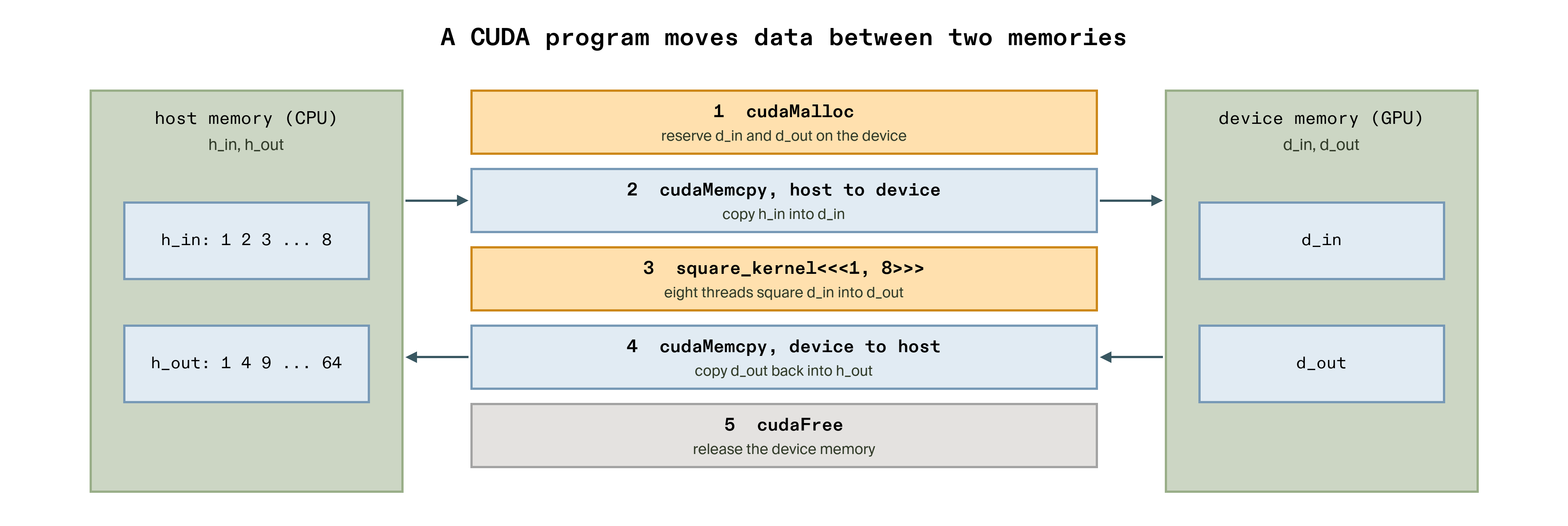
There are two new CUDA functions here, both from the CUDA runtime API. cudaMalloc() allocates memory in the device's global memory and gives us a pointer to it. cudaMemcpy() copies bytes between host and device memory. The final argument tells CUDA which direction the data should move: cudaMemcpyHostToDevice for the input and cudaMemcpyDeviceToHost for the result.

The naming convention h_ for host data and d_ for device data is not required by CUDA, but it is a useful convention because both are represented as pointers in C++. Keeping the distinction visible helps us remember where each piece of data lives.

The kernel receives d_in and d_out as arguments, and each of the eight threads squares the single element that its threadIdx.x points at. This is the data parallelism from the previous section, now written as a real kernel.

The if (i < n) check may look unnecessary because we launched exactly eight threads for eight elements. We include it because, once we start launching blocks with a fixed number of threads, the total number of threads will not always match the number of elements exactly. The check prevents threads whose indices fall outside the array from accessing memory they do not own. Running the program gives:

   1 squared is    1
   2 squared is    4
   3 squared is    9
   4 squared is   16
   5 squared is   25
   6 squared is   36
   7 squared is   49
   8 squared is   64

Frameworks such as PyTorch manage much of this memory handling for us. When we create a tensor with device="cuda", PyTorch allocates storage for that tensor in GPU memory. Operations on CUDA tensors then launch kernels that operate on that device-resident data. When we call .cpu() on a CUDA tensor, PyTorch transfers its contents back to CPU memory.

CUDA gives us direct control over these steps. That makes the code more verbose, but it also lets us see something that frameworks usually hide: where our data lives, when it moves, and which processor is operating on it.

Launches are asynchronous

There is a detail in the squaring program that is easy to miss. When the host launches a kernel, it does not normally wait for that kernel to finish. The launch queues the work for the GPU and returns control to the host, allowing the CPU to continue executing the next statement while the GPU works independently.

The next operation was a cudaMemcpy() from device to host. That copy waits for the required earlier GPU work to complete before returning the result to the host. By the time we print h_out, the kernel has finished and the results have been copied back.

In our earlier hello program, there was no device-to-host copy to create that waiting point. That is why we explicitly called cudaDeviceSynchronize(), which blocks the host until previously issued GPU work has completed. Without it, main() could reach the end while GPU work was still outstanding.

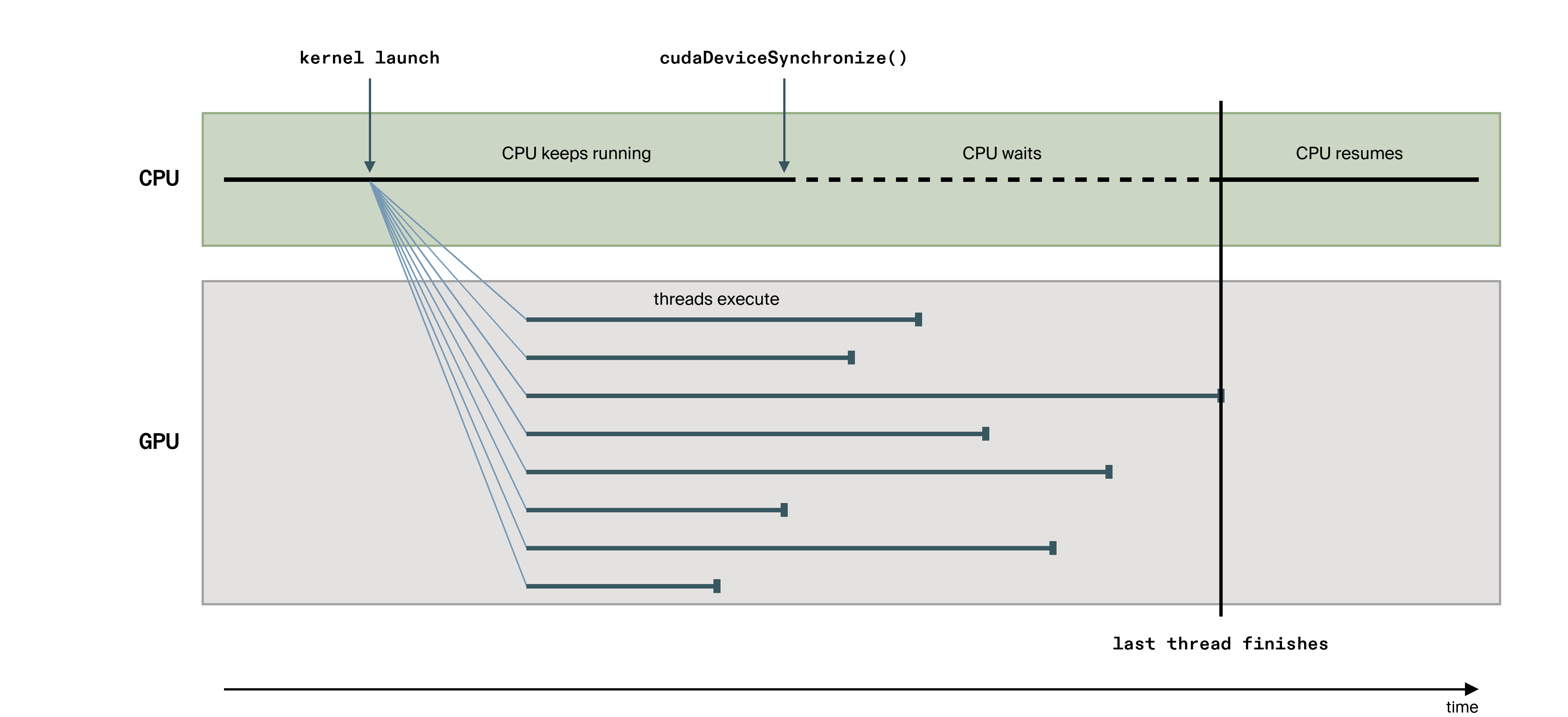
PyTorch launches are asynchronous in exactly the same way, and this has a practical consequence for anyone who tries to time GPU code. If we wrap an operation in time.time(), the elapsed time is the cost of issuing the launch on the CPU side and says nothing about how long the GPU spent on the kernel. To measure the kernel, the CPU has to wait for the GPU first:

import time
import torch

a = torch.randn(50_000_000, device="cuda")
b = torch.randn(50_000_000, device="cuda")
a + b                         # warm up
torch.cuda.synchronize()

t0 = time.time()
c = a + b
t_launch = time.time() - t0   # how long the CPU spent issuing the work

torch.cuda.synchronize()      # block until the GPU has finished all queued work
t_done = time.time() - t0     # how long the GPU actually took, plus the launch

print(f"launch returned after {t_launch * 1e6:7.0f} us")
print(f"work finished after   {t_done * 1e6:7.0f} us")

On our L40S we got this:

launch returned after      25 us
work finished after       993 us

‍This difference is the key idea: launching GPU work and completing GPU work are two different events, and only the second one tells us how long a kernel took.

Operations that require data on the CPU create synchronization points as well. For example, calling .cpu() on a CUDA tensor must make the requested tensor data available in CPU memory, and .item() must retrieve a scalar value before Python can use it. This is why synchronization matters when measuring GPU programs. Without it, we may accidentally measure how quickly the CPU can submit work rather than how quickly the GPU can finish it.

From one block to many blocks

Our squaring program used a single block, which was fine for eight elements. It cannot work for a million, because a block is limited to 1,024 threads on current NVIDIA GPUs. The limit exists because the threads of a block are guaranteed to run on the same SM, where they can share that SM's fast memory and coordinate with one another, and an SM only has the resources to track so many threads at once. To process a large array we launch many blocks, and the whole collection of blocks created by one launch is called the grid.

So the hierarchy has three levels. A grid contains blocks, a block contains threads, and, as we saw, the hardware executes those threads in warps of 32. There are now two related hierarchies to keep in mind.

1. Software, how we organize the work: grid → blocks → threads
2. Hardware, how the GPU executes that work: threads → warps → SMs

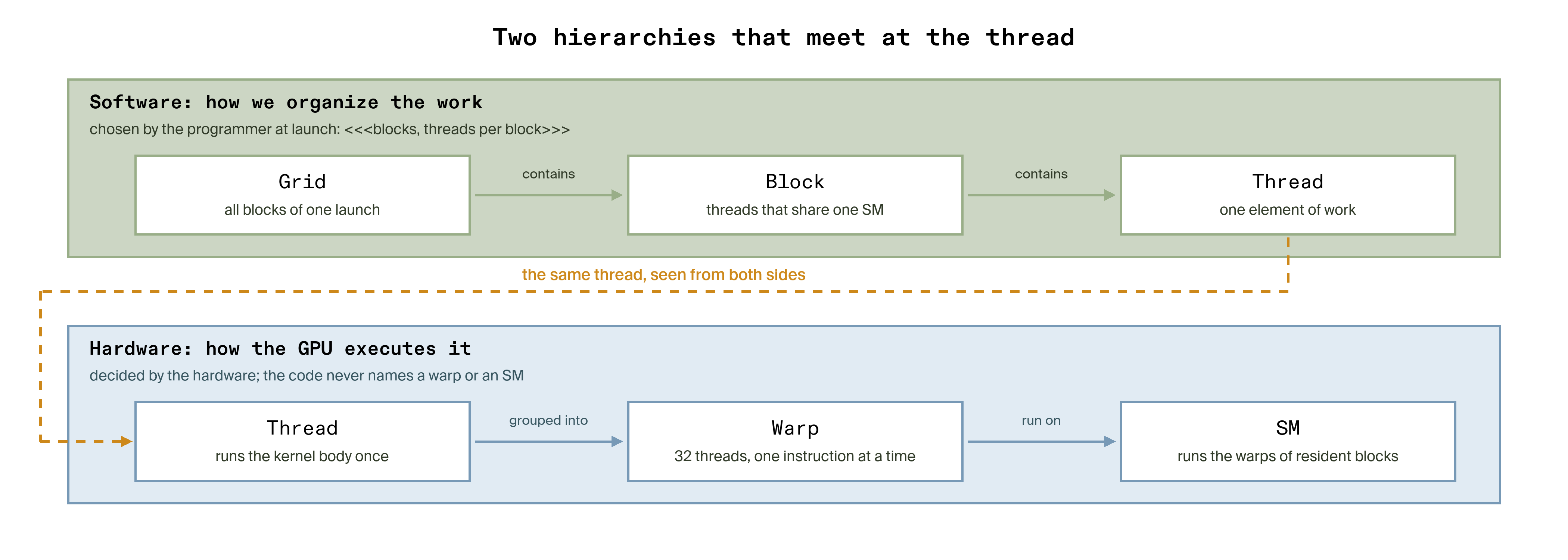
The grid is a purely logical description of how much work exists. Nothing in the grid specifies which SM will end up running which block, and because of that the same kernel can be launched unchanged on GPUs of very different sizes.

Finding the right element

Introducing more than one block creates a problem. The variable threadIdx.x restarts at zero in every block, so if we launched three blocks of four threads and used threadIdx.x as the element index, all three blocks would work on elements 0 to 3 and elements 4 to 11 would never be touched. Each thread needs to know not only its position in its block but also which block it is in.

CUDA provides that through two more built-in variables. blockIdx.x is the block's position in the grid, and blockDim.x is the number of threads per block, the second number in the launch syntax. We can combine these with threadIdx.x to calculate a thread's global index across the entire grid:

int i = blockIdx.x * blockDim.x + threadIdx.x;

The formula skips over all the elements handled by earlier blocks, then adds the thread's position within its own block. It is similar to identifying a seat in a theater with numbered rows: the row number tells us how many full rows to skip, and the seat's position within that row tells us how far to move into the current row.

How many blocks, and how big

Two decisions remain: how many threads per block, and therefore how many blocks. Suppose we settle on 256 threads per block and have one million elements to process. One million divided by 256 is 3,906.25, and we cannot launch a quarter of a block. Rounding down would leave 64 elements unprocessed, so we round up to 3,907 blocks, which is written in integer arithmetic as:

int blocks = (n + threads_per_block - 1) / threads_per_block;

Rounding up means the grid now contains 3,907 × 256 = 1,000,192 threads, which is 192 more than we have elements. Those extra threads live in the last block, and their computed index i is 1,000,000 or above. Without a guard they would access memory beyond the end of our arrays and corrupt whatever happens to sit there. This is why the if (i < n) check from the squaring program is not optional: an input length seldom divides evenly by the block size, so the final block almost always extends past the end of the array, and every kernel must check before it touches memory.

Why 256 rather than some other number? The warp is the unit the hardware actually schedules, so a block should be a multiple of 32; a block of 250 threads would still occupy 8 warps, with 6 lanes of the last warp doing nothing. Block size also affects how many blocks and warps can be resident on an SM at the same time, along with other factors such as register and shared-memory usage. There is no single best block size for every kernel, but 128 to 256 threads per block is a good starting range, and 256 is a sensible default that we will use throughout. We will see why these choices matter once we look more closely at how the GPU keeps enough work in flight.

The complete kernel

Putting the pieces together gives the general form of an elementwise CUDA kernel. This is vector addition, the very operation PyTorch launched for us when we wrote a + b at the start of this part, and the kernel we will write again in Triton at the end of it:

__global__ void add_kernel(const float* x, const float* y, float* out, int n) {
    int i = blockIdx.x * blockDim.x + threadIdx.x;   // global element index
    if (i < n) {                                     // last block may overrun
        out[i] = x[i] + y[i];
    }
}

// On the host:
int block = 256;
int grid = (n + block - 1) / block;                  // ceiling division
add_kernel<<<grid, block>>>(d_x, d_y, d_out, n);

You can find the full code in the Crusoe Developer Hub. The example checks the result against a CPU loop, then times the kernel with CUDA events, which record timestamps on the GPU's own timeline and therefore measure kernel execution rather than the CPU issuing the launch. Before each timed launch it writes a 256 MB scratch buffer, for a reason we explain below, then reports the median of fifty runs and converts the time to bandwidth by counting three arrays of four-byte floats. On our L40S:

Running on NVIDIA L40S

    elements   blocks  median ms       GB/s    check
        1000        4     0.0041        2.9       OK
       65536      256     0.0061      128.7       OK
     1048576     4096     0.0205      614.4       OK
    16777216    65536     0.3123      644.7       OK

‍Every size passes the correctness check, including the first one, where 1,000 elements do not divide evenly into blocks of 256 and the guard is doing its job. The timing column rewards a closer look. For 1,000 elements the GPU has almost no work to do, so the 4 microseconds we measure is essentially the fixed cost of a launch, and the bandwidth figure is meaningless. As the arrays grow the kernel becomes worth launching, and from one million elements upward it moves data at 614 to 645 GB/s, roughly 75 percent of the 864 GB/s the L40S's global memory is rated for.

Now for that 256 MB scratch buffer. When we first wrote this program without it, the one-million-element row reported 2,048 GB/s, more than twice what global memory can deliver, and no kernel can read faster than the memory it reads from. The data was coming from somewhere closer. Three arrays of one million floats occupy 12 MB, and the L40S has a 96 MiB cache, called the L2 cache, sitting between the SMs and global memory. After the first of the fifty timed repetitions the whole working set was in that cache, and the other forty-nine never touched DRAM at all. Writing 256 MB of unrelated data before each launch pushes our arrays out of the cache, so every repetition has to fetch them from global memory again and the table reports the memory, not the cache. At 16 million elements the working set is 192 MB and would not have fit anyway, which is why that row barely changes.

There is a general lesson here that we will rely on throughout the series: timing a kernel repeatedly on a small input measures the cache unless you deliberately evict it. Triton's own benchmarking helper does the same eviction, and we will use it from the next part onward. The next section places the L2 cache among the other levels of GPU memory.

Where blocks run

We now have 3,907 blocks and, on the L40S, 142 SMs to run them on. Each SM can hold several blocks at once, as long as their combined demands for registers and on-chip memory fit within what the SM has.

A launch of 3,907 blocks is therefore not executed all at once. A hardware scheduler places blocks on SMs that have free capacity, and as blocks complete, waiting blocks take the freed slots, until every block in the grid has run.

Three properties of this arrangement shape how every kernel is written.

1. A block runs on a single SM from start to finish and is never moved. This is what makes it possible for the threads of a block to share on-chip memory and to synchronize: they are physically together on one SM for the block's whole lifetime.
2. Blocks run in no particular order. The scheduler gives no guarantee that block 1 starts before block 7 or finishes before it, and correct code cannot depend on any ordering.
3. Blocks cannot rely on direct synchronization with one another during an ordinary kernel. There is no mechanism for block 3 to wait for a value from block 9, because block 9 may not be resident yet, and with a large grid it may not become resident until block 3 has finished. When a computation needs a result that depends on every block, such as the total of an entire array, it is either split across two kernel launches or done with special atomic operations on global memory, and we will use both approaches when we get to reductions.

These constraints are the price of portability. Because blocks are independent, the same kernel runs unchanged on a GPU with 40 SMs and on one with 140, the smaller GPU simply takes more rounds to work through the grid.

The numbers for the GPU in front of us are available from PyTorch, and it is worth printing them once. The script in the GitHub repo also works through our one-million-element example:

GPU                       NVIDIA L40S
Streaming multiprocessors 142
Warp size                 32 threads
Max threads per SM        1536
Warp slots per SM         48
Global memory             44 GiB
L2 cache                  96 MiB
Compute capability        8.9

1,000,000 elements at 256 threads per block
  blocks in the grid      3,907
  warps in the grid       31,256
  warp slots on the GPU   6,816  (142 SMs x 48)
  waves, at best          4.6

‍Each SM on this GPU can hold 1,536 threads, which is 48 warps, so across 142 SMs at most 6,816 warps are resident at any moment. Our grid has 31,256 warps, about 4.6 times the GPU's maximum number of resident warp slots. The phrase "at best" is there because a kernel that uses many registers per thread fits fewer warps on an SM than the hardware maximum, and the next section explains why that matters.

The memory hierarchy

GPU memory is not a single pool with a single access cost. It is organized as a hierarchy, with small, fast storage close to the execution units and progressively larger, slower memory farther away. Arithmetic instructions operate on values held in registers, so every value has to travel from wherever it is stored to the execution units before it can be used, and the cost of that trip depends entirely on where the value started. Where data lives, and how often it moves between these levels, is therefore the main determinant of a kernel's speed.

At the top are registers. Registers are private to a thread and are where arithmetic instructions get their operands and place their results. Values such as i and the loaded values of x[i] and y[i] in our kernel are held in registers while the thread operates on them.

Next is shared memory, a small region of fast on-chip memory that threads within a block can use to exchange and reuse data. This is the fast memory we mentioned earlier when explaining why a block stays on one SM. The L1 cache is also located close to the SM, but unlike shared memory it is managed automatically by the hardware.

Below that is the L2 cache, which is shared across the GPU's SMs and sits between the SMs and global memory. Data accessed from global memory can be cached here, allowing later accesses to be served without going all the way back to DRAM. This is the 96 MiB cache that held our 12 MB working set in the vector addition timing above, and the reason the program evicts it before every timed launch.

Then comes global memory, the large DRAM where our CUDA arrays and PyTorch tensors normally live. Its aggregate bandwidth is enormous, but any individual access has to wait several hundred clock cycles for its data, compared with roughly one cycle for a value already in a register and tens of cycles for shared memory. That ratio of a few hundred to one is the single most important number in GPU performance, and the five trips through global memory in the first figure of this part were all on the expensive side of it.

Finally, data that lives in host memory may need to travel between the CPU and GPU across the host-device interconnect, as we saw with cudaMemcpy().

Latency hiding and occupancy

If a single load from global memory takes hundreds of cycles, a fair question is how a GPU accomplishes anything. The answer is that it does not try to make an individual access fast. Instead it keeps a large number of warps resident on each SM, and when one warp issues a load and has to wait, the scheduler switches to another warp whose data has already arrived. With enough warps in rotation, the arithmetic units stay busy even though every single warp spends most of its time waiting.

This is one reason a GPU wants far more threads in flight than it can execute at any single instant. The extra warps give the scheduler other work to choose from when some warps are stalled. CPUs also try to hide latency using mechanisms such as caches, out-of-order execution, and speculation; GPUs rely heavily on having many threads and warps available to run.

But the number of warps that can be resident on an SM is limited by hardware resources. Every thread needs registers, and every block may require shared memory. A kernel that uses many registers per thread or a large amount of shared memory per block may therefore allow fewer blocks, and consequently fewer warps, to reside on an SM at the same time.

The fraction of the maximum supported warps on an SM that are actually resident is called occupancy. For example, we saw that an L40S SM can support up to 48 resident warps. If the resource requirements of a kernel allow only 24 warps to be resident, its occupancy is:

24 resident warps / 48 maximum warps = 50% occupancy

Introduction to GPU programming with Triton

A reasonable question at this point is what Triton adds over the CUDA we have just used. The short answer is that it moves the level at which we write from the thread to the block; the longer answer starts with what Triton is.

Triton is a domain-specific language, or DSL, for writing GPU kernels. A DSL is a small language designed for one kind of problem rather than for general programming SQL for database queries and regular expressions for text patterns are familiar examples, and both are standalone languages with their own syntax. Triton is instead an embedded DSL: it borrows Python's syntax and lives inside Python programs. To write a Triton kernel we write a normal Python function and place the @triton.jit decorator above it, and launching it looks like any other Python function call. Python has several such embedded languages. Numba compiles decorated Python functions to native CPU machine code, and JAX traces Python functions into a computation graph that it then compiles. In each case the function looks like Python and sits alongside ordinary Python, but something other than the Python interpreter ends up executing it.

Triton includes both a compiler and a runtime. The compiler takes the body of the decorated function and translates it, through several intermediate stages, into the same kind of GPU machine code that nvcc produces from CUDA C++. The runtime handles everything around that: it triggers compilation the first time a kernel is called with a new combination of argument types, caches the result so later calls skip straight to launching, and launches the compiled kernel on the device with the grid we ask for. Both are installed as part of the Triton package. In our environment, Triton was already available alongside PyTorch.

Where Triton sits is easiest to see against the two things we have already used. PyTorch gives us whole operations and hides the GPU entirely; CUDA gives us every thread and every byte, and asks us to manage them. Triton occupies the space between. We describe the computation we want performed on a block of data, and the compiler makes the decisions that in CUDA would be ours: how the threads share the work, how memory accesses are arranged so that neighboring threads touch neighboring addresses, when shared memory is worth using, and where synchronization is needed. Each of those decisions affects performance, and later in the series we will look at what the compiler chooses and why. For this part, the point is that they are no longer written by hand.

The Triton programming model

The one conceptual shift that matters when coming to Triton from CUDA is this: we write programs for blocks, not for threads.

Recall what the CUDA version of vector addition asked of us. The work was organized in two tiers, a grid of blocks and a block of threads, and the code we wrote was the program for a single thread. That thread computed its own element index from blockIdx.x, blockDim.x and threadIdx.x, checked that the index was in range, and handled one element. Any coordination between threads, such as sharing data through the SM's on-chip memory or waiting for one another, would also have been ours to write.

Triton removes the need to coordinate threads by hand. A Triton kernel is written from the point of view of a single program instance, and that instance operates on an entire block of data rather than on one element. We decompose the task into one level only, the block. Triton's compiler and runtime decide how the individual threads inside that block carry out the instructions, and shared memory is handled for us automatically. Because a program instance works on a whole block at once, its operations are naturally vectorized: loading, computing, storing and masking all act on vectors rather than on individual scalars. This one-tiered design is what makes the programming model simpler, and it is why the kernel we are about to read has no thread index anywhere in it.

A small example makes the difference concrete. Suppose x and y each hold eight numbers and we want z = x + y, and suppose we choose a block size of four, so the work splits into two blocks. In CUDA we launch two blocks of four threads, and each of the eight threads computes one output, such as z[0] = x[0] + y[0].

In Triton we launch two program instances, and each one computes four outputs as a single vector operation: the first evaluates z[0:4] = x[0:4] + y[0:4], the second z[4:8] = x[4:8] + y[4:8]. Whether that vector operation becomes one hardware instruction or several is the compiler's concern, not ours.

This way of thinking tends to feel natural quickly, because most numerical work already comes in blocks. Matrices are processed as tiles, images as channels, long vectors as segments. Triton lets us write the computation for one such block in plain vector operations and leaves the thread-level bookkeeping to the compiler, which is exactly the part of CUDA programming that is easiest to get wrong and slowest to debug.

Same program, many blocks: SPMD

The pattern that makes the block-level view work has a name. In the single program, multiple data (SPMD) model, many instances of one program run the same code, and each instance handles its own portion of the data. We have already been using it: the CUDA kernels in this part were one program run by thousands of threads, each on its own element. SPMD is older than GPUs; it is how programs written for message-passing and shared-memory clusters have been structured for decades.

It is worth keeping SPMD separate from SIMT, which we discussed when we looked at warps.

• SPMD describes how the program is written: one body of code, applied to many pieces of data.
• SIMT describes how NVIDIA hardware executes it: threads gathered into warps, one instruction issued to the whole warp at a time.

The first is a property of our source code, the second a property of the machine.

Triton keeps the SPMD pattern and changes only its granularity. Instead of one worker per element, we have one program instance per block of elements, and the same instructions apply across the whole block. We write the computation for one block, specify a grid that launches one program instance per block, and each instance locates its own portion of the input from the program ID that the launch assigns to it. Underneath, the hardware still runs warps on SMs exactly as described earlier; the compiler is what maps our block-level program onto them.

With that model in place we can write our first Triton kernel, and the natural choice is the same one we used for CUDA. Vector addition is the closest thing parallel computing has to a "Hello, World!" program: the data flow is obvious, every element is independent, and it maps directly onto the block-level view.

Here is the kernel from the repo, alongside the host code that launches it.

import torch
import triton
import triton.language as tl

@triton.jit
def add_kernel(x_ptr, y_ptr, output_ptr, n_elements, BLOCK_SIZE: tl.constexpr):
    pid = tl.program_id(axis=0)                   # which program instance am I?
    block_start = pid * BLOCK_SIZE
    offsets = block_start + tl.arange(0, BLOCK_SIZE)
    mask = offsets < n_elements                   # guard for the final instance

    x = tl.load(x_ptr + offsets, mask=mask)       # global memory to registers
    y = tl.load(y_ptr + offsets, mask=mask)
    tl.store(output_ptr + offsets, x + y, mask=mask)

def add(x, y):
    output = torch.empty_like(x)
    n = x.numel()
    grid = (triton.cdiv(n, 1024),)                # ceiling division, as before
    add_kernel[grid](x, y, output, n, BLOCK_SIZE=1024)

    return output

‍Every line has a counterpart in the CUDA kernel we wrote a few sections ago, and reading them side by side is the best way to see what has been abstracted.

The most important difference is what is missing: there is no threadIdx.x.

Instead, tl.program_id(axis=0) tells us which program instance is running. From that ID we calculate block_start, and tl.arange() creates a vector of offsets:

program 0 → offsets    0 ... 1023
program 1 → offsets 1024 ... 2047
program 2 → offsets 2048 ... 3071
...

‍Each program instance therefore operates on a block of elements at once, and the mask given to tl.load() and tl.store() keeps the final instance from touching positions past the end of the tensor, exactly as if (i < n) did in CUDA.

The script launches this kernel for several input lengths, including one that deliberately leaves a partial final block, and compares every result with PyTorch's own addition:

Running on cuda:0 - NVIDIA L40S

size=         1  OK
size=       128  OK
size=      1024  OK
size=   1048583  OK

‍There is one final connection back to where we started. In the opening section we counted two kernel launches and five array-sized trips through global memory for (a + b).relu(), and we said we would return to what happens when the two operations are brought together. The count_kernels.py script in the repo does exactly that on our L40S. It runs the expression once in eager mode and once through torch.compile, and asks the profiler how many kernels ran and how long each one took:‍

eager: 2 kernel(s), 6.656 us on the GPU
     3.680 us  void at::native::vectorized_elementwise_kernel<4, at::nat...
     2.976 us  void at::native::vectorized_elementwise_kernel<4, at::nat...

torch.compile: 1 kernel(s), 3.392 us on the GPU
     3.392 us  triton_poi_fused_add_relu_0

‍The two eager rows above are the kernels we saw in the profiler table, the add and the clamp behind ReLU. With torch.compile, PyTorch fused the addition and the ReLU into a single GPU kernel. That kernel reads a and b once and writes c once, three trips through global memory instead of five, with one launch instead of two. The timing shows the payoff: the fused kernel finishes in 3.392 us, roughly half of the 6.656 us the two eager kernels take together (which we saw earlier). Its name, triton_poi_fused_add_relu_0, tells us how it was made.

PyTorch's compiler stack can generate Triton kernels as part of optimizing GPU workloads. By learning Triton ourselves, we gain the ability to write and tune specialized kernels directly when we want more control over how an operation is implemented. That is the level of abstraction we will work at for the rest of this series.

Summary

We started with a single line of PyTorch and followed it all the way down to the GPU.

Along the way, we saw how GPU work is expressed as kernels, how threads are organized into warps and blocks, how blocks are scheduled across SMs, and how data moves through the GPU's memory hierarchy. We also saw why GPUs keep many warps in flight to hide memory latency.

Most importantly, we wrote the same vector addition in both CUDA and Triton. CUDA made the underlying execution model explicit: thread indices, blocks, bounds checks, memory allocation, and kernel launches. Triton let us express the same computation at the level of blocks of data while leaving much of the thread-level mapping to the compiler.

These concepts do not disappear when we use Triton. Threads, warps, SMs, registers, caches, and global memory are still the hardware underneath our program, and understanding them gives us the vocabulary to reason about why a Triton kernel behaves the way it does. That vocabulary is what the rest of the series builds on.

Run the code

All code from this part is available in the GPU Engineering section of the Crusoe Developer Hub.

The repository contains the CUDA examples, the Triton vector-add kernel, profiler scripts, benchmarking code, and instructions for creating the environment and running everything on a Crusoe GPU.

To follow along on Crusoe, create a GPU VM from the Crusoe Cloud console. A single-GPU instance is enough to run the examples in this series. We used an NVIDIA L40S for the measurements in this part, but you can use another supported NVIDIA GPU as well.

Once the VM is running, connect to it over SSH, clone the Crusoe Developer Hub repository, and follow the README for the latest environment and setup instructions. The Python scripts only need the environment the README creates. The CUDA C++ examples also need the CUDA toolkit for the nvcc compiler, and the README shows how to install it.

Next in the series

In the next part, we will take the Triton vector-add kernel apart properly. We will look at tl.constexpr, BLOCK_SIZE, program instances, grids, compilation, and the intermediate representations generated by Triton. We will also establish the benchmarking approach we will use throughout the rest of the series.

From there, we can start doing what this series is really about: writing Triton kernels, measuring them, and understanding why they perform the way they do.

References

• NVIDIA, CUDA C++ Programming Guide: the sections on the thread hierarchy, memory hierarchy, and SIMT architecture underpin the execution model described here.
• NVIDIA, CUDA C++ Best Practices Guide: occupancy and GPU memory performance.
• NVIDIA, An Even Easier Introduction to CUDA: an introduction to CUDA programming that builds vector addition from a single thread to a grid of threads.
• OpenAI, Triton documentation: the programming model, language reference, and tutorials for writing Triton kernels.
• Crusoe Developer Hub, GPU Programming with Triton: companion code for this series.
• Crusoe, Creating and Managing GPU VMs: instructions for creating and managing the GPU instances used to follow along with the series.