AutoClusters: Minimizing the impact of hardware failures in large GPU clusters

Hardware failures in large GPU clusters are routine events. For the most expensive AI workloads like distributed training, a single GPU being unavailable can halt a training run and force you to roll back to the last checkpoint. The result is enormous costs incurred via lost work and idle GPU time.

This dynamic presents a critical engineering challenge: how do you design systems that gracefully handle these routine failures while minimizing impact to your workloads? This post covers the economics of GPU failures, the variables you can control, and how Crusoe Cloud built AutoClusters to solve the problem. 

How often do failures occur?

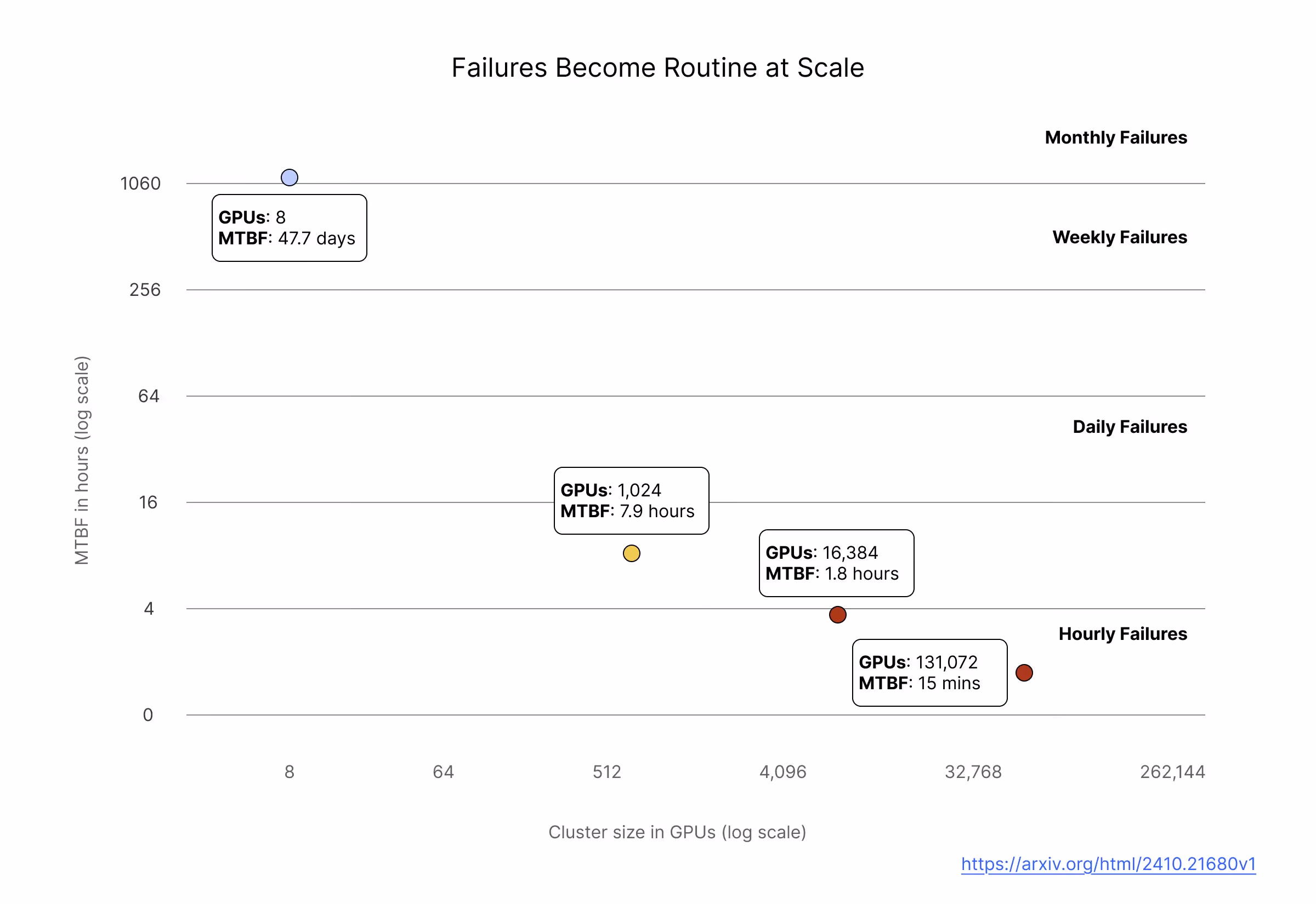
Meta published detailed data on failures across their research clusters, analyzing 150 million hours of A100 GPU usage [1]. At 8 GPUs, mean time between failures (MTBF) is around 47 days, which is manageable with ad hoc human intervention. At 1,024 GPUs, MTBF drops to about 8 hours, meaning you're dealing with failures multiple times per day. At 16,384 GPUs, MTBF is around 1.8 hours.

There is an inverse relationship between cluster size and MTBF. This relationship is intuitively understood, since more components means more opportunities for something to go wrong, but the practical implications are significant. At large scale, failures are so frequent that manual investigation and correction is unsustainable. Automated detection and remediation is required because humans simply can’t respond fast enough to multiple incidents per day without severely diminishing the amount of useful work the cluster is able to complete.

The distribution of failure impact is also uneven. Meta found that while failures affected only 0.2% of jobs overall, they consumed 18.7% of total runtime because large, long-running jobs encounter failures more often and each failure wastes many GPU hours.

What’s eating your goodput?

Your contract with a GPU cloud provider specifies a cost per GPU hour, but your real target outcome is useful work: jobs that finish with minimal time wasted. The industry term for this is “goodput”: the fraction of your compute time spent doing useful work versus overhead.

Goodput gets eaten by checkpoint overhead, work lost to rollbacks, time waiting for replacement nodes when nodes fail, and compute inefficiencies that slow your workload to below its theoretical peak. We can express goodput as a function of these variables:

G = (1 - (c + f + q)) x e

In this equation:

• c is checkpoint overhead, the fraction of time spent saving state instead of training
• f is failure loss, the fraction of work time lost when you roll back to the last checkpoint
• q is queue wait, the fraction of time spent waiting for replacement nodes
• e is compute efficiency, how close your workload runs to its theoretical peak

Note that failure rate does not appear directly in this equation, but it is a key driver of other terms. Failure rate determines your optimal checkpoint frequency (which sets checkpoint overhead), how much work you lose when a failure occurs and you have to roll back to the prior checkpoint (failure loss), and how often you pay the queue wait penalty. We will detail this relationship shortly.

What goodput factors can you actually control?

The factors that determine goodput are not equally controllable, and understanding which levers you can pull is the key to thinking clearly about the economics of GPU failures.

Compute efficiency depends primarily on your own engineering work, such as kernel optimization, data loading pipelines, and batch size tuning. A competent provider supplies well-configured hardware with proper drivers and network setup, but past that baseline, efficiency gains come from your side.

Checkpoint overhead and failure loss are coupled through a fundamental tradeoff: checkpointing more frequently reduces work lost per failure but increases time spent saving state. The optimal interval depends on failure rate and checkpoint duration (it is roughly proportional to the square root of MTBF multiplied by checkpoint cost). Once you've optimized your infrastructure to speed up checkpoint operations (fast storage, efficient serialization, tiered writes to memory), the remaining overhead is derived from your failure rate.

‍Failure rate is partially controllable with diminishing returns. Good providers reduce it through burn-in testing, active health checks, and proactive replacement of degrading hardware. But hardware still fails. You can push failure rates down, but not eliminate them.

Queue wait depends on how quickly failed nodes get replaced. You can manage this yourself with spare capacity and automation, or rely on your provider's remediation infrastructure. When a node fails, your job sits idle until a replacement is available. With manual intervention, that wait time can be 60-120 minutes. With automated detection and a warm spare pool, it can be 5-10 minutes, possibly lower if you optimize heavily. That's an order of magnitude difference, and you pay it on every failure.

Failure patterns in GPU clusters

To understand what good detection and remediation looks like, it helps to understand how hardware actually fails, because different failure patterns require different responses.

Sudden failures

Some failures are binary and there's no ambiguity about what happened. A GPU falls off the PCIe bus, reports a critical hardware error, or becomes completely unresponsive. The node is effectively bricked with replacement being the only path forward. These sudden failures are easy to detect, so the challenge is purely replacement speed.

Gradual degradation

Other failures develop over time in ways that are harder to catch. A GPU might be accumulating ECC memory errors, and while a single correctable error is normal, when correctable errors start clustering it usually indicates the high-bandwidth memory is beginning to fail. If you wait for uncorrectable errors, you've already impacted a workload.

Thermal issues follow a similar pattern. A GPU that's occasionally throttling due to high temperatures might still report as healthy in basic monitoring, but it's delivering less compute than you're paying for. Sometimes this indicates a failing component on that specific node, and sometimes it's a datacenter cooling issue affecting a whole section of machines.

The common thread is that catching gradual degradation requires more than passive monitoring. You need active health checks that exercise hardware under realistic load, not just check whether it responds to basic queries.

Lemon nodes

This is a particularly frustrating pattern that only becomes visible when you're operating at scale. Some nodes pass health checks when idle but fail under real workloads. They get marked as bad after a job fails, get replaced, pass health checks and get scheduled for another job, only to fail again. Without systematic tracking, these nodes cycle through your fleet indefinitely, wasting time on every job that has the misfortune of landing on them.

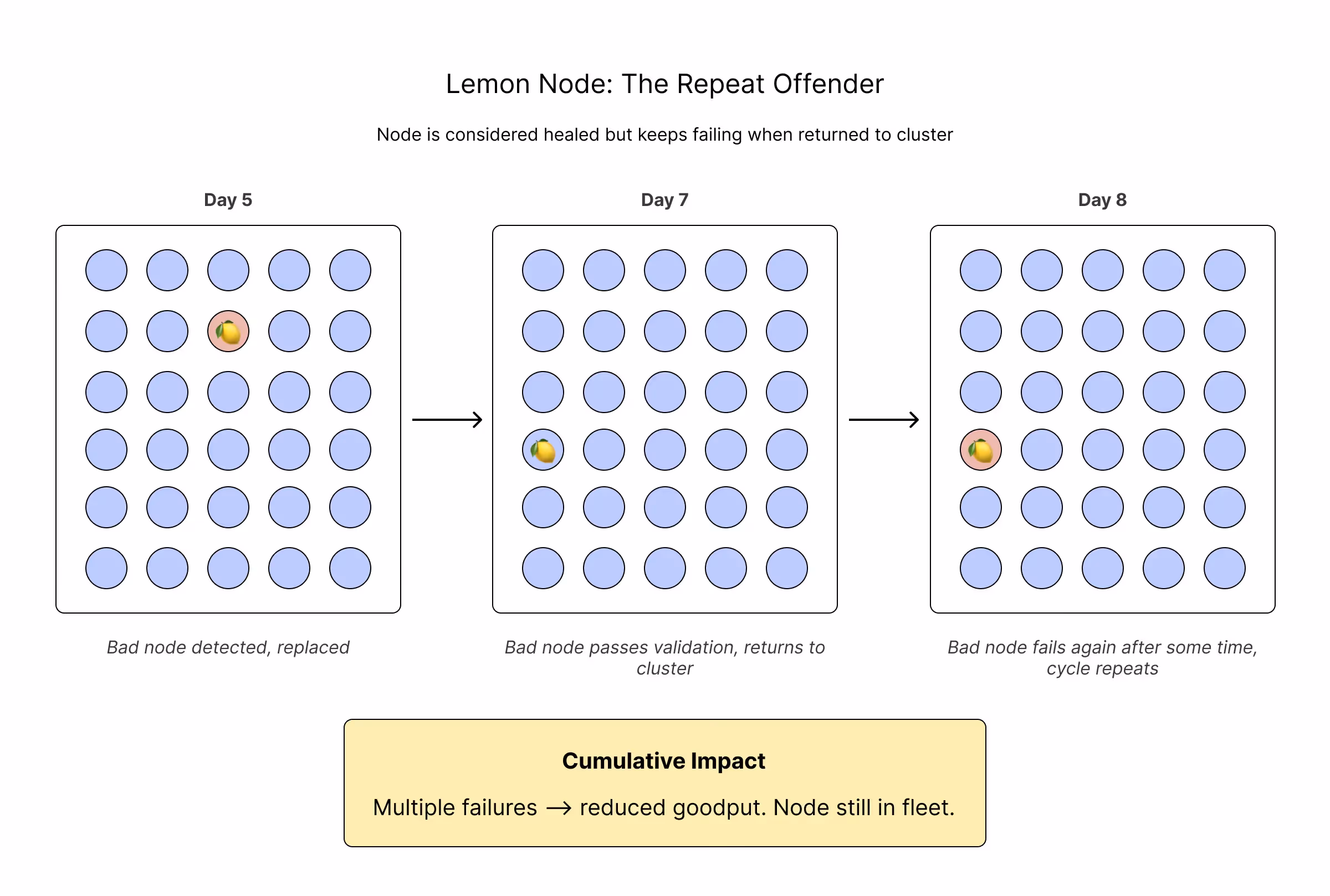
The root causes span the hardware stack, including GPU issues, memory failures, PCIe problems, network interface issues, and firmware bugs. The common thread is that the problems don't manifest under synthetic health check workloads, only under real production load. When Meta implemented systematic lemon node detection and removed these nodes from scheduling, failure rates for large jobs dropped from 14% to 4% [1]. That's a dramatic improvement from simply identifying and excluding the nodes that repeatedly cause problems.

Correlated failures

Individual component failures are manageable. What's dangerous is when a single root cause takes out multiple nodes at once. A failing network switch can disconnect dozens of nodes simultaneously. A power distribution unit problem can drop an entire rack. And a bad driver update pushed fleet-wide can cause widespread GPU errors.

This matters for automation design. If one node fails, automatic replacement is the right response. But if multiple nodes in the same rack fail simultaneously, something upstream probably needs human investigation, and naive automation that just starts replacing nodes can make the situation worse by churning through your spare pool while the actual problem persists.

The cost of failure: a worked example

Consider a 1,000 GPU training cluster. Based on the MTBF data discussed earlier, we can expect a failure every 8 hours on average, or 3 failures a day. Assume your checkpoint infrastructure is optimized to run checkpoints in 1 minute, and you have calculated that the optimal checkpoint frequency is once every 30 minutes. For the purposes of this example, let’s assume you’ve optimized compute efficiency such that it is 100% of potential.

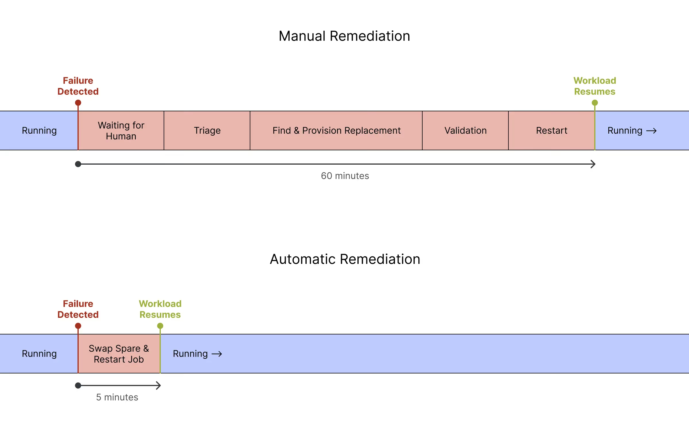
Also assume that you have a purely manual, 60 minute remediation process. Each time a failure occurs, the following happens:

1. A failure occurs, and your job hangs
2. An alert fires, and an engineer gets paged (5-30 minutes depending on time of day)
3. The engineer triages which node failed and why (10-20 minutes)
4. The engineer goes through a manual workflow to cordon the bad node, drain workloads, and find and provision a replacement (20-40 minutes)
5. The engineer runs validation on the replacement node (10-15 minutes)
6. The job is restarted (5-10 minutes)

Here is how the above scenario translates to lost work over a 24 hour period.

Checkpointing every 30 minutes implies 48 checkpoints. At one minute per checkpoint, that’s 48 minutes total, about 3% of the 24 hour period. 

With 30-minute checkpoint intervals, you lose an average of 15 minutes of work per failure (half the interval) by rolling back to the last checkpoint. Three failures means 45 minutes lost, roughly 3% of the period.

With each failure costing you 60 minutes in manual remediation, you pay 180 minutes in queue wait time, about 12.5% of the period.

Adding it all up, over a 24 hour period, you spend 273 minutes, or 19% of time, not doing any useful work, giving you a goodput of 81%

Obviously, after experiencing a few of these incidents, you will look to optimize your queue wait time by speeding up your remediation flow. There are a number of opportunities to move faster. For example, you can have better alerting so you immediately know what action to take. You can script the replacement process to run automatically. You can keep a warm pool of pre-validated nodes to eliminate the validation step before you resume your job. Taken to its logical conclusion, you end up with fully automated remediation.

To illustrate, let’s assume the exact same scenario, but replace the manual remediation workflow with an automatic remediation workflow. Now, each time a failure occurs, the following happens:

1. A failure occurs, and your job hangs. The automated remediation workflow detects the failure and kicks off the remediation workflow. (30 seconds)
2. The failed node is automatically cordoned so it stops accepting new workloads (Immediate)
3. Running workloads get a configurable grace period to checkpoint and terminate cleanly via a container preStop hook. (30 seconds)
4. A known-good node from the spare pool joins the cluster. Because spares are pre-validated during burn-in, there's no extensive health verification step needed at replacement time. (4 minutes)
5. The orchestrator automatically assigns work to the new capacity (Immediate)

The checkpoint cost and failure loss stay the same at 48 minutes and 45 minutes, respectively. But your queue wait time drops from 180 minutes to just 15 minutes. Now your total time lost to failure is just 108 minutes, or 7% of the total time period. That improves goodput to 92%, an 11% improvement.

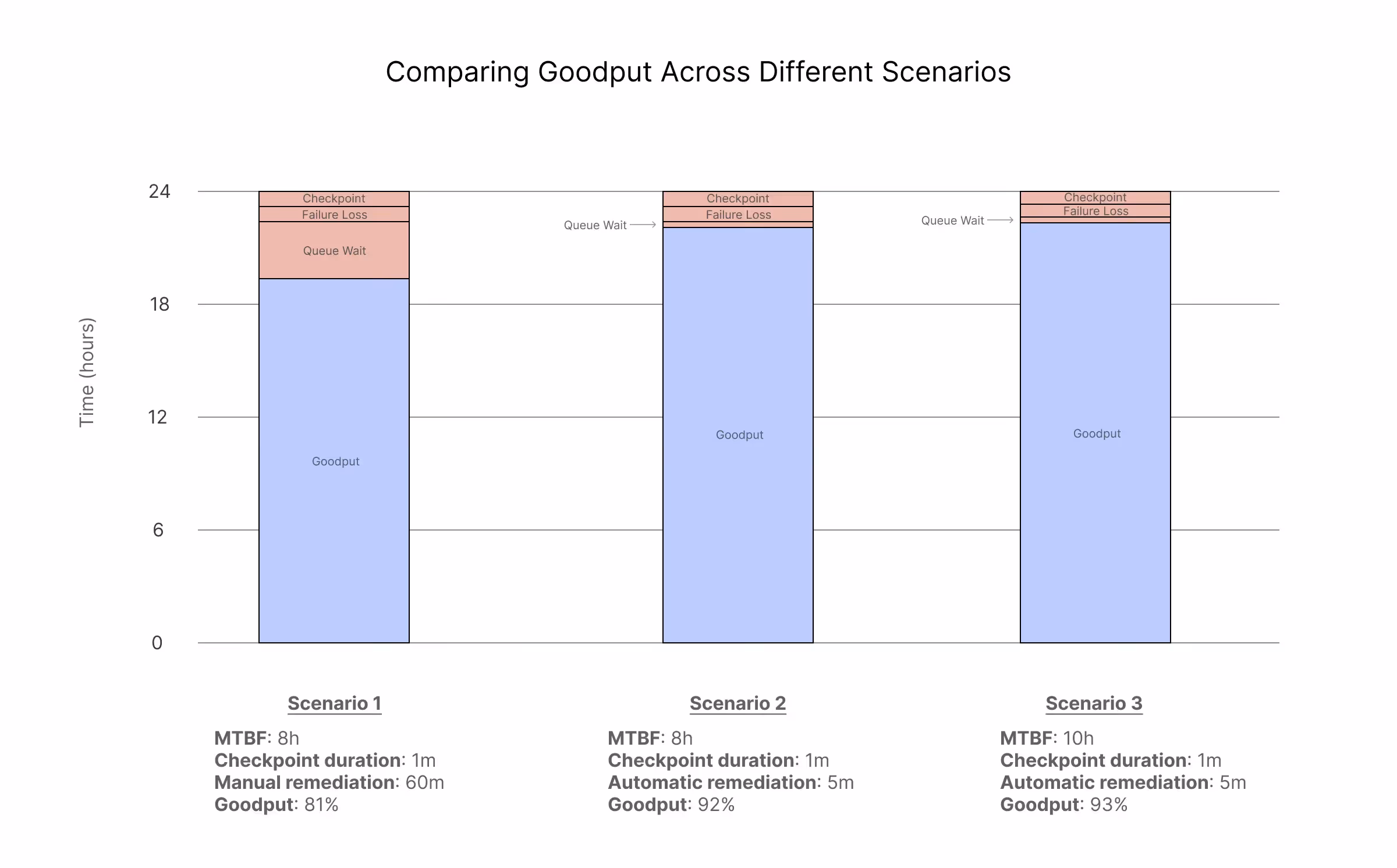
Note that failure rates do vary by cloud provider, and a lower rate of failure can also improve goodput, but not by the same magnitude as replacing manual remediation with automatic remediation. In the same scenario above with automatic remediation, consider an improvement that results in an MTBF of 10 hours instead of 8 hours. The optimal checkpoint interval changes to 35 minutes. The arithmetic is left to the reader, but the final goodput is 93% vs 92%. Better, but not a dramatic jump.

What makes remediation fast?

Saying “we have fast automated remediation” is easy, but building infrastructure that consistently delivers 5-minute replacement times is harder. It is worth understanding what goes into this, both to appreciate the engineering effort involved and to know what questions to ask when evaluating cloud providers.

Spare pool management

Fast replacement requires a pool of pre-validated spare nodes ready to go. You can't provision on demand and hit 5-minute replacement times, since provisioning alone takes longer than that.

The sizing question is nontrivial. With too few spares, a burst of failures exhausts your pool. With too many, you leave potential training throughput on the table. The right ratio depends on cluster size and failure patterns.

Placement matters too. If all your spares are in one rack and that rack loses power, your backup capacity is gone exactly when you need it. Spares need topological diversity.

And spares can't just sit idle indefinitely. Hardware degrades and firmware gets stale, so the spares need regular health cycling to ensure they're actually ready when called upon.

Detection speed

You can't replace a failed node until you know it failed. Passive monitoring catches obvious failures (a node that stops responding or a GPU that reports a critical error). But as discussed earlier, gradual degradation and lemon nodes require active health checks that exercise hardware under realistic load.

The challenge is distinguishing signal from noise. A brief network blip, a temporary thermal spike, or a transient error that clears on retry shouldn't trigger replacement. Good detection tracks patterns over time rather than reacting to single data points.

Correlation detection

When one node fails, automatic replacement is the correct action. But when several nodes in the same rack fail within a minute, something upstream is broken (a switch, a power event, or a bad config push). Blindly replacing all nodes exhausts your spare pool while the actual problem persists.

This requires tracking not just that failures occurred, but where and when. Failures clustered in time and topology suggest a shared root cause, and the right response is to pause automation and escalate for human investigation.

The replacement flow

Even with spares ready and failures detected instantly, the mechanics take time: cordon the failed node, drain running workloads (giving jobs time to checkpoint), select a matching spare, provision it into the cluster, run a final health validation, and resume workloads. Each step has latency. Getting total time under 5 minutes requires optimizing all of them.

How AutoClusters works

AutoClusters is our implementation of these principles for workloads running on Crusoe Managed Kubernetes. Our approach has three layers: validation before nodes enter your cluster, continuous monitoring while they're running, and fast remediation when problems occur.

Validation before provisioning

Before a node is ever available for scheduling in your cluster, it goes through burn-in testing. We run GPU stress tests, memory checks, and network validation to catch hardware that's dead on arrival or unreliable. Nodes that don't pass burn-in never enter your available pool.

Nodes that pass go into a warm spare pool, already validated and ready to swap in when a failure occurs. This is why automated remediation can be fast. We're not provisioning and validating on demand. We're pulling from a pool of known-good hardware.

Detection

Once nodes are in your cluster, we run continuous passive monitoring of GPU telemetry through DCGM, logs, PCIe status, and network fabric health. This catches sudden failures: nodes that stop responding, GPUs that report critical errors.

We're extending this with periodic active health checks that exercise hardware under real load, catching subtle degradation that passive monitoring misses. 

Remediation

When a failure is detected, the default behavior is automatic node replacement from our spare pool. The failed node is cordoned immediately so it stops accepting new workloads. Running workloads get a configurable grace period to checkpoint and terminate cleanly (default 30 seconds). A known-good node from the spare pool joins the cluster. 

Because spares are pre-validated during burn-in, there's no additional health verification at replacement time. This takes about 4 minutes. The orchestrator then assigns work to the new capacity immediately.

Total time from failure detection to a replacement node ready for work is typically under 5 minutes.

Correlation detection and circuit breakers

Not all failure patterns should trigger automatic remediation. If a single node fails, replacement is the right response. But if many nodes in the same rack or network segment fail simultaneously, something bigger is probably going on: a bad switch, a power event, a problematic driver update.

To prevent remediation storms where a shared root cause triggers a cascade of replacements, we've implemented circuit breakers that pause automation when failure patterns look anomalous. If too many nodes in a cluster fail within a short window, we stop automatic remediations and alert for human investigation. This is live today.

Visibility

All of this is visible through the Crusoe Cloud Console. You can see every remediation event: what triggered it, which node was involved, what replacement node was provisioned, and how long the process took.

What’s next for AutoClusters?

We're extending AutoClusters with capabilities that address even more failure patterns and give you more control over remediation workflows. Here's what's coming:

Lemon node detection 

Our active health checks will include systematic lemon node detection — when we see repeated failures on the same hardware, we'll remove it from rotation permanently rather than letting it cycle back into your pool. 

In-place remediation 

Node replacement is the reliable backstop, but not always the fastest path to recovery. For certain failure modes, in-place remediation can restore a node in seconds. We're building a library of in-place fixes for common patterns, with node replacement as the fallback. 

Open-loop remediation

Some workloads have operational requirements that need custom handling when failures occur. Maybe you need to checkpoint to a specific location before a node is removed, notify an external system, or run application-specific validation. 

For these cases, we're building open-loop remediation. Instead of AutoClusters automatically replacing the node, failure events are exposed to your automation. You consume these events, run whatever custom logic you need, and then call our remediation API to trigger replacement. This gives you the benefit of our detection and replacement infrastructure while maintaining control over the workflow.

What about inference workloads?

This post focused on training because that's where checkpoint, failure loss, and queue wait dynamics are most complex. A single GPU failure halts a synchronized training job entirely, and all workers must wait for the failed node to be replaced.

Inference is different because a single failure doesn't halt everything. But you do lose capacity and tail latency degrades until you replace the node. The same principle applies: faster remediation means less time running at degraded capacity, fewer latency spikes for your users, and less risk of cascading failures when you're running near capacity limits.

Conclusion

When you're running GPUs at scale, most of what determines your goodput is either in your hands (your code, your kernels, your checkpoint infrastructure) or subject to diminishing returns given the realities of hardware. The exception is queue wait. That's pure dead time, determined entirely by detection and remediation capabilities.

A provider with automated detection, warm spare pools, and fast replacement will deliver meaningfully better goodput than one relying on manual or slow remediation. The math is straightforward, and the difference compounds with every failure. Learn more about Crusoe AutoClusters.

Citations

1. Pinckney, N., Cai, H., Wu, C., Tanaka, Y., Chiang, P., Huang, J., ... & Asanović, K. (2024). "Revisiting Reliability in Large-Scale Machine Learning Research Clusters." arXiv:2410.21680. [Link]

‍